An introduction to parsing and BNF, and why you should care even if you’re not writing a compiler

Parsing tasks are extremely common and even though major efforts have been done to standardize our inter-systems communications we still end up analyzing various text files which have structure – but not a structure that we have a library at hand that can parse. As an example, say you have something that outputs this sort of text (I assume this isn’t a real format, it’s not supposed to be).

fruits {
    banana {
        [tasty="true"]
        [colour="yellow"]
    }

    orange {
    }
    
    [eatable="if not rotten"]
}

How would you go about it, if you want to store the output result in some form of object? I often see splitting on spaces, and other characters, making convoluted paths and abusing regular expressions to no end to wrangle these sorts of things into whatever data structure you have on your client. What if I said there is a better way. It’s not new by a long short, but it rarely spreads outside of advanced comp-sci classes or compiler designer classes to the more pragmatic programmers working in the real world.

Grammars

There’s generic tools that can parse these sorts of texts. They’re incredibly efficient at doing this as well. They simply require the right input. That input is a grammar. A grammar is really the set of rules that a text must follow in order to be parseable. For instance, in the example above we could assume that it would be illegal to not match the brackets properly, or to have an unnamed node. The way of expressing grammars is known as the Backus-Naur form, or BNF for short. It’s an easy syntax.

Resulting symbol := List of input symbols | Another list of symbols | [maybe an empty section as well];

A symbol is one of two things. It’s either a terminal symbol or a nonterminal symbol. Terminal symbols are those that are directly translatable from the input, nonterminals are built up from lists of other symbols – both terminal and nonterminal ones. Lets start to make a grammar for our input.

To make it easy on ourselves, we’ll simplify the input text and add features in as we go. Let’s start with identifying only this subset

basenode {
}

There are three distinct terminal tokens here: name, { and }. Note that the terminal name will represent for us all the legal nodenames. It’s typical that a terminal token is defined by a regular expression. Let’s assume that name can be only lowercase alphabetic characters. The only legal combination of these terminals are is name followed by { followed by }. This must yield a non terminal token. Let’s call it object. The grammar will look like this:

terminal name [a-z]+

object := name '{' '}' ;

A few things about this grammar, for shortness it allows single character terminal to be used as is. Standard regex notation defines the terminal to be lowercase a-z, repeated at least once.

Lets add the [attribute=”value”] notation next. A sample of legal input is now:

rickastley {
    [nevergonnaone="give you up"]
    [nevergonnatwo="let you down"]
    [nevergonnathree="run around"]
    [nevergonnafour="and desert you"]
}

Now it gets more interesting, since there can be more than one attribute, and maybe zero. This is where the cool recursive nature of grammars come into play. Looking at the notation of attributes, we can see that we will require four more terminals: [, ], = and a quoted-string. We will also require three more non-terminals: attribute, attribute-list and optional-attribute-list. I’ll give you the grammar, and we can discuss why it looks like it does.

terminal name [a-z]+
terminal quoted-string "[^"]+"

object := name '{' optional-attribute-list '}' ;

optional-attribute-list := attribute-list 
                         | ;

attribute-list := attribute-list attribute 
                | attribute;

attribute := '[' name '=' quoted-string ']'

I like to pronounce := as is-made-up-of. Using that, lets analyze the rules:

1. An object is made up by name followed by an optional-attribute-list enclosed in bracers
2. An optional-attribute-list is made up of either an attribute-list or nothing. The nothing part is important, since this is what makes the rule optional.
3. An attribute-list is an attribute-list followed by an attribute, or just an attribute. This sort of self-recursion is key to understanding formal grammars. A list is either a single item, or another list with another item tacked on to the end. This is probably all very familiar if you know functional languages like lisp (cons)
4. An attribute is simply some terminals tacked together to form a nonterminal called attribute.

The grammar above will recognize an object with any number of attributes, including none, using recursion.

Adding the child objects is similar. This time we will not require any new terminals. We will require two new non-terminals: optional-object-list and object-list.

terminal name [a-z]+
terminal quoted-string "[^"]+"

object := name '{' optional-object-list optional-attribute-list '}' ;

optional-object-lit := object-list 
                     | ;

object-list := object-list object 
             | object ;

optional-attribute-list := attribute-list 
                        | ;

attribute-list := attribute-list attribute 
                | attribute ;

attribute := '[' name '=' quoted-string ']';

As you can see, the object list refers to the main rule object, which causes all the same rules applied to the main object to be applied to the child objects as well. This recursive feature of grammars is extremely powerful. So, we have reduced this problem down to 8 lines of grammar, which save for a few changes in syntax is entirely compatible for a whole range of parser generators.

In fact, more often than not when you are reading text you are in fact parsing it. Only when reading text that has no real context, like counting words without caring if they are nouns or verbs are you not parsing. So why do we keep writing text parsing code by hand when we have all this power right at our fingertips?

This question has been the main motivator for me behind writing Piglet, my parser generator. Not to replace any of the large full-featured generators out there, but to provide a small and nimble alternative that can be easily embedded into your application. Democratizing the formal grammars if you will. It’s currently near an alpha state, with runnable code and a reasonably efficient generation. Feel free to contribute, it’s on github. I’ve also updated the Demo project to include an implementation of this particular grammar. The curious reader will perhaps wonder why there currently are two implementations of the same stuff. That’s because Piglet tries to be educational and chatty and supports a fluent interface for configuration which has a few convenience methods for making lists and optional things. The implementation that exactly matches the non-extended grammar shown in this post is the second method.

If you study the grammar above there are a few things that could be improved. For instance, you must specify child objects first, before specifying attributes. If you’re interested enough, try modifying the grammar so that this becomes possible. It’s good exercise!

I hope I’ve gotten you at least a bit interested in how parsing using tools really works. Hopefully an introductory post for my own library isn’t too far away so it can be put to the test. This little series on parsing will continue with more technical details on how these parsing tools actually work.

How to handle WPF events in native MFC code

I’ve recently had the dubious pleasure of getting to know C++/CLI and revisiting my good old buddy MFC. The task at hand was to integrate a WPF component into an existing MFC application. That task in itself is probably interesting enough to warrant it’s own post but suffice to say that I got this working properly. This means that we’ll end up with a class deriving CDialog that holds a WPF component inside it. Now we want to handle events. In WPF country, this is easy: add this to our WPF class:

public event EventHandler OnMyEvent;

And in our dialog we hold the WPF control in a gcroot<MyWPFControlClassName>. We also have a method we’d like to get called.

void MyDialogClass::OnEvent(System::Object ^sender, System::EventArgs ^args)
{
   // Do stuff
}

First off, what prompted this article is what does not work. You cannot from your unmanaged dialog class pass a pointer to your member function to your event like this.

wpfControl->OnMyEvent += gcnew System::EventHandler(
      this, 
      &MyNativeDialogClass::OnEvent);

This does not work, and it’s because your class is not a managed class since it’s not declared as ref class. The error message is also less than helpful. So how to solve this? You need a wrapper. Create this class somewhere in your project.

#pragma once

template<class T> ref class ManagedEventWrapper {
public:
   typedef void(T::*MemberFunction)(System::Object^ sender, System::EventArgs^ args);

   ManagedEventWrapper(T& host, MemberFunction function)
      : m_host (host)
      , m_function(function) 
   {
   }
   
   void OnEvent(System::Object ^sender, System::EventArgs ^args)
   {
      (m_host.*m_function)(sender, args);
   }

private:
   T& m_host;
   MemberFunction m_function;
};

If you then include this file in your MFC class, then you can subscribe to events like this:

wpfControl->OnMyEvent += gcnew System::EventHandler(
      gcnew ManagedEventWrapper<MyNativeDialogClass>(*this, &MyNativeDialogClass::OnEvent), 
      &ManagedEventWrapper<MyNativeDialogClass>::OnEvent);

This creates the neccessary layer of extra indirection around the native code to make the event handling work properly. You don’t need to save the reference to ManagedEventWraper since the reference is held by the System::EventHandler which makes sure it does not get garbage collected.

Drawing graphs with graphviz

If you’ve read any of my posts regarding regular expressions you’ve seen these little graphs. I just wanted to tell you all how they were made. They might not be very pretty, but it’s easy to produce them, especially programmatically from source code. In fact, it’s so easy that I’ve included graph output as a standard debugging feature in my parser generator. And they can get quite pretty indeed, if you know what you’re supposed to do.

This is part of a library called GraphViz. Unfortunately the graphviz tool set is about as user friendly as a bicycle without a saddle attached. Well, they do have a GvEdit application that you can input stuff in and get a graph. I suggest using this online tool and just right-click to save your graphs. That’s what I do anyway.

I find it remarkable what you can achieve with this tool, and I use it more and more since I loathe to draw and layout things by hand. A basic directed graph looks like this:

digraph g {
  a -> b
  b -> c
  c -> a
}

If you want more nodes, just add them in and draw arrows. Easy. The engine will lay this out for you and present you with a pretty picture. I’m by no means an expert, but I have gathered a few tricks (use inside of the brackets unless stated otherwise).

• Graphviz likes to draw with arrows pointing downwards. Use graph [rankdir="LR"] to make it tend to draw left to right instead
• Change the default node shape by adding node [shape="whatever shape you want"]. Theres a few to choose from, in my graphs i used circle and doublecircle
• Add lables to your little arrows by adding [label=”xx”] after the end node.
• Whichever node you define first will tend to be drawn to the upper left

This is the tip of the iceberg really, graphviz.org has lots more information. As long as you don’t try to position the nodes manually you’re pretty much good to go. It really is a tool for getting graphs without having to do all the cumbersome work with moving stuff around to make it pretty. If you need fine grained per-pixel control, this isn’t for you. If you need to get a graph up and running quickly and to modify it easily, this tool should be right up your alley.

Converting a DFA to a table, Regular expressions part 3

So, last time we explored the wonderful world of regular expressions we ended on a nice looking graph representing our deterministic machine that recognized the regular expression that generated it. That’s all fine, but in reality we’d like a table representation for our machine. Tables offer some significant benefits, most prominently they’re really fast with O(1) access times. They are, however, not very compact. That flaw can be remedied with table compression though, which I will not delve into in this post. Mostly because I do not completely understand it yet.

Anyway, here’s where we ended up last time:

First order of business is to assign state numbers to each state. It’s really arbitrary what numbers you give the states as long as they are unique, but keeping with tradition we’re going to assign 0 to the starting state. The graph now looks like this:

Now we can create a table. On the X-axis we will use the character input, on the Y axis we will use the state number. For each state, if there is a transition to another state using a given input character, we fill in the state number to go to in the corresponding column. If the state is an accept state, add a special ACC for accept. The table will look like this:

           INPUT 
------+---+---+---+---+
STATE | a | b | c | d |
------+---+---+---+---+
  0   | 1 | 2 |   |   |
------+---+---+---+---+
  1   | 1 | 2 |   |   |
------+---+---+---+---+
  2   | 1 | 3 |   |   |
------+---+---+---+---+
  3   | 2 | 3 | 4 |   |
------+---+---+---+---+
  4   |   |   |   |ACC|
------+---+---+---+---+

Apply the pseudocode algorithm outlined in the first post to this table, and you’ve got your very own regular expression engine!

Wrapping up, there’s of course more to do. This engine does not handle things such as capture groups, lookahead and all that advanced stuff. But it isn’t that hard to add, and nothing of what’s been said will not hold true for the more full-featured engines. Another option is to never do the table generation stuff and instead emit actual IL code that will execute the DFA straight up, which would be incredibly cool stuff. As I said earlier these tables end to be very sparse, since the input requited normally is at least 256 different characters and only a few are legal for each state. This means that there’s a lot to do on the compression side as well.

If there’s any questions or requests for elaborations on all of this, I’ll happily accept and answer. Otherwise, I think it’s time to continue with regular expressions big brother – parsers.

Converting a NFA to a DFA by subset construction, Regular expressions part 2

Welcome again to the understanding regular expressions series, the previous part is located here if you missed it. Much like the dragon book you probably really can’t read these things out of order. Last time we ended with a really nice non deterministic finite automata, but in order to make it work in a deterministic fashion we will need to transform it. Again, a deterministic machine is the mirror image of a nondeterministic machine, it will achieve exactly the same thing but in a different fashion.

For reference, a nondeterministic finite automata:

• One entry state
• May contain epsilon transitions
• One input may lead to several new states
• One accepting state

It’s cousin the deterministic finite automata (DFA) has these properties:

• One entry state
• May not contain epsilon transition
• One input may only lead to one state
• May have several accepting states

The key thing about the DFA is that we can easily convert it to a table and run it through our very simple engine, giving us very nice run-times of O(n). So how to convert this machine? The algorithm used here is called closure and it is very cool indeed. It is also used in a different variation for parser generation, which is why it’s almost a must to understand regular expressions before starting to truly understand parser generators. Here it is

Given a list of states the closure set is all the sets that can be reached without any input, including the input states themselves

The function will have an input of one or more states, and return a set of states which will at least contain the input states. In pseudo C# code it looks like this. I myself much prefer pseudocode that is much closer to real code – it leaves much less to the imagination of the reader.

Set<State> Closure(List<State> inputStates)
{
    var output = new Set<State>();
    output.AddRange(inputStates);

    // Keeps states we are going to add later
    while (true) 
    {
        var statesToAdd = new Set<State>();
        foreach (var state in output)
        {
            foreach (var edge in output.EdgesGoingOut)
            {
                if (edge.IsEpsilonEdge)
                {
                    if (!output.Contains(statesToAdd)) 
                    {
                        statesToAdd.Add(edge.DestinationState);
                    }
                }
            }
        }
        if (!statesToAdd.Any())
            break; // Exit loop if there are no states to add
        output.UnionWith(statesToAdd); // Add all states to output
    }
    return output;
}

It’s helpful to visualize this using graphs. If we return to the regular expression (a|b)+bcd, the corresponding NFA looks like this

If we are going to compute closure for state 0 we will traverse the edges to 1 and 3, but not to 5, because that edge goes the wrong way. Then there are nowhere else to go, since the remaining transitions require inputs “a” or “b” respectively. So the closure of state 0 is {0, 1, 3}. Note that the input state is always included in the closure list. I like to think of this as a flood fill, because it looks like that if you have many epsilon transitions. This new set is actually the start of our deterministic machine! Yay. Lets begin to draw the machine to watch it grow.

Our first state

We now need to introduce a new operation called goto. I know, goto is a bad word these days. The algorithm apologizes profoundly for the association. The goto algorithm is real easy.

Given a set of states and an input symbol find all the states reachable by traversing the edges that require the given input symbol. Then apply the closure algorithm on the output

Think of this algorithm as move one step then flood fill again. In C# pseudocode it looks like this

List<State> Goto(List<State> inputState, char inputCharacter)
{
     var output = new Set<State>();
    foreach (var state in inputState)
    {
        foreach (var edge in state.EdgesGoingOut)
        {
            if (edge.Label == inputCharacter)
            {
                output.Add(edge.DestinationState);
            }
        }
    }
    return Closure(output);
}

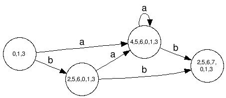
So, given our first closure set {0, 1, 3} lets apply Goto on it for every input character. Nothing will happen except for characters “a” and “b”. Lets explore character “a”. The only transition we get to cross is the one going from state 3 to 4. So 4 is the only result of the Goto. We now apply closure to it, which gives us the list {4, 5, 6, 0, 1, 3} when we follow every arrow which is an epsilon. The input for “b” is very similar and yields state set {2, 5, 6, 0, 1, 3}. The next step is adding our new states to the new diagram with the input we gave to the Goto as the edge label. Now the graph looks like this:

You then repeat this again. Applying Goto on the state set {4, 5, 6, 0, 1, 3} and input “a” gives us exacly the same result as previously. This means that this state has an edge going to itself. Applying Goto on the same states with input “b” gives a new state set that we haven’t seen before {2, 5, 6, 7, 0, 1, 3}. Lets add this to our graph:

If we apply the same algorithm to the state list {2, 5, 6, 0, 1, 3} we find that it will only yield sets that we have already added to the graph, but it will give us new transitions. The graph now looks like this:

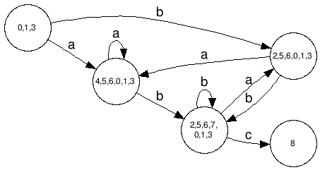
There is one unexplored set to apply goto on {2, 5, 6, 7, 0, 1, 3}. Doing this with “a” gets a transition back to a previously known state. “b” gives a transition back to the same state list. “c” gives a transition to a brand new set containing only state 8. Our graph now looks like this:

Still one new set to explore! Only one input gives a new set “d” gives a set containing only state 9. State 9 is an accepting state, so we add this to the graph.

Applying goto on this new set gives us nothing at all. We are done. Almost by magic we have transformed our non-deteministic machine into a deterministic machine. The reader is invited to try the same input as on the nondeterministic variant. It will respond the same. There is really only one bit left to do, we need to make this into a table that will run with our regular expression engine.

Next part can be found here

One of the coolest books I have ever read

If you’re even a tiny bit like me, you want to know how things work. And I don’t mean in the sense of “I know how a car works because I can drive it”. No, I mean in the sense that you know how the car works because you understand the internal combustion engine, the clutch and the differential axle – at least on a conceptual level. I’m also going to assume you sort of like computers, at least you’re reading this using one aren’t you. Have you understood how they work on a conceptual level?

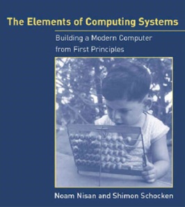
This book is about that, and boy does it do a good job. The book in question carries the unassuming name of The Elements of Computing Systems and looks about as boring as it possibly could. But the contents are a whole different matter. Reading the book and doing the exercises will have you building a computer from the ground up.

The book starts by explaining what a logical gate is and how to construct other gates from a given gate. It has you building all the necessary gates out of NAND gates. It goes ever more complex, you build multiplexers, memory, a full adder, an ALU, a CPU – all with quite excellent tools that the book has freely available on it’s companion site.

It doesn’t stop there, once the computer is done it proceeds with writing your own very simple assembler for your home-made assembly language. In which you write a simple compiler for your home-made assembly on your home made computer. In which you carry on writing a very simple operating system for your computer. If that doesn’t blow ones mind away, what will?

The thing about this book is that it will never involve anything in the realm of electrical engineering. There are no talks of transistors and other stuff, which isn’t really necessary either to grasp the concepts. Reading this book is a truly eye-opening experience, and you simply won’t look at a computer the same way again.

Oh, and did I mention that most of the book actually is quite freely available from it’s companion site?

If this isn’t enough to convince you of how awesome this book is, the things inside it will enable you to build this sort of crazy stuff:

Regular expressions, how do they really work? Automata theory for programmers part 1

I know, automata theory doesn’t sound like the most exiting thing on earth, but there’s more than meets the eye here. I’m going to assume you have at least a working knowledge of regular expressions. You don’t need to worry about knowing the intricate little details to appreciate this article. So, let’s get going.

If you think regular expressions are some sort of glorified wildcard, you’re wrong. They are more akin to mathematical expressions than anything else, which is also why they’re called expressions. For the sake of completeness they are called regular because they can implement any regular (type 3) grammar on the Chomsky language hierarchy. To understand how they actually work, you have to understand what a state machine is.

State machines

In the most common sense, a state machine is something that holds a given state, and have transitions to other states based on some conditional, usually input. It’s a very useful concept. It’s commonly implemented as a loop with a switch statement at the base, switching on the current state. For each state, the machine performs given actions which might result in the machine changing state. This in turn will reflect in it’s next iteration. Regular expressions are typically parsed by state machines. Each iteration takes an input, and evaluates it based on the current state of the machine – advancing it to either a new state, an error state or an accept state (i.e. the string has matched the expression). State machines for regular expressions are typically driven by tables.

This is pretty much all you need to know to implement the actual engine. It looks a bit like this:

bool Matches(Reader r)
{
   int state = 0;
   while (r.Peek() != -1)
   {
      char input = (char)r.Read();
      if (table[state, input] == Accept)
          return true; // Table indicates that for this state, we accept the input given
      if (table[state, input] == Error)
          return false; // Table indicates that this is not a valid input
      // Advance to next state.
      state = table[state, input];
   }
}

Really, that is it. The engine that drives regular expressions is pretty much this. As you can see, all the complexity are in the construction of the tables. Because the tables can be constructed beforehand the actual regular expression evaluation can be extremely fast. So, what we’re going to be mainly discussing are how to construct these tables. To do this we’ll have to define our state machines in a different way, and introduce a few cool new terms.

Nondeterministic Finite automata

It sounds fancy, but it’s really our friend the state machine all over again but this time with a twist. A nondeterministic finite automata is a state machine that may advance it’s state without an input and be in more than one state at the same time. Like a quantum state machine. A transition between two states in this fashion is called an Epsilon transition. I like to think that E stands for empty. The thing about these state machines is that it’s a lot easier to construct them than it is to construct their deterministic cousins. It’s especially easy to combine them, as we shall see.

Deterministic finite automata

State machines which require some sort of input on every state, and where the same input in one given state can never lead to two different places. This has two effects, it’s always clear what to do given an input and you’re always in only one state at a time. Two highly desirable characteristics indeed.

Constructing nondeteministic finite automata

It’s easy enough to show this by some drawing. A circle is a state, identified by a number. A double circle is an accept state – a state where we consider the expression to be matched if we are at the end of the input. An arrow is a transition between states. The text on the arrow is the required input to transfer the machine from one state to another.

The simplest one of them all, this machine accepts a single “x” character.

This machine first takes an “x” then an “y” then accepts the input.

Both of these machines are by nature deterministic, they cannot be in more than one state at a time, since there are no epsilon transitions. For an example of that, take a look at this machine

Note that there is an epsilon transition in this one, represented by the funny-looking e character. This means that this transition is automatic. This machine will match the strings “y” or “xy”. When starting the machine will be state 1 from which it detects an epsilon transition and follows it automatically while still being in state 1. So, now we’ve got a machine that is in both state 1 and 2. Depending on the input different things will now happen. If we get an “y” the machine that is in state 1 will have nowhere to go, and since machines must always advance on input this machine will die – leaving only the machine in state 2 which can continue to state 3 and accept the input. The reverse thing happens if an “x” were inputted. In that case the machine in state 1 dies since it can’t go anywhere, leaving the other machine to advance to state 3.

It’s not that hard to figure out how to translate different elements in regular expressions to these small machines. Here’s a few more examples:

Accepts “x” zero or more times. Equivalent to the expression x*

Accepts “x” one or more times. Equivalent to the expression x+

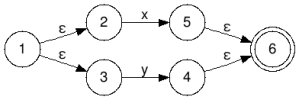
Accepts either “x” or “y”. Equivalent to the expression x|y

The amazing thing about these machines is that you can string them together into a huge machine, they are infitely combineable. As long as you stick to the rule about a single starting state and a single accept state. You’ve already seen two examples of this, the machine that accepted “xy” was two machines each accepting a single character linked together. The other example is the last example which accepted either “x” or “y”, liked together by alternation. To construct these compound machines the easiest way is to convert the regular expression into postfix notation and apply a stack based algorithm. Both of these are really not that difficult algorithms, but this post is long enough as it is. It’s briefly explained in this document. It’s also quite well documented in the source code of my parser generator Piglet, look at the classes NFA and PostFixConverter. If there’s interest in further explanation of this, I’ll see if I can write something up.

Turns out there aren’t that many ways to link machines together for basic use, most have already been shown here. So, as a final example here is a machine that accepts the regexp (a|b)+bcd

Try following the edges and keep track of machines that are alive for the various forms of inputs. It will do exactly what you want given the regexp. And it’s all built on combinations of the same building blocks shown above. So, given these tools you could actually construct a machine that accepts any regular expression. However, these machines are not very efficient since they need to keep track of multiple states which given a large enough expression could be quite cumbersome. We still want to have that desireable deterministic effect, where we could just keep track of one state and know where to go for each given input.

That is probably going to be the next part of this algorithmic exploration!

Edit: Next part can be viewed here

Tales of extreme debugging

Sometimes debugging, at least through the rose-tinted goggles of hindsight can be quite amusing. Today I’m going to share with you two of the better ones I’ve experienced myself to brighten up your day. I don’t really know if there’s any wisdom to be drawn from them, but they’re true and fun.

It’s too cold outside to debug

Back in late -04 early -05 I was working for Gizmondo programming games. This wasn’t exactly by choice, since our studio was bought by them we just sort of ended up doing games for this unit that was supposed to be the next big thing. Turned out it became a big thing for all the wrong reasons. So, I was one of the precious few people who actually got to develop on this machine, and while it might have been a miserable failure in some points it was groundbreaking in others. One thing was that this little device actually included a GPS chip. Now kids, this is way before the first iPhone so this was quite a novelty. I had this stint with some talented guys to make the client side of this multiplayer game Colors, which was to be the first GPS multiplayer game in the world. The gist of it was that you could control neighborhoods by actually going there and challenging the current ruler. So, being the client side guy I set out on a task to implement this.

If there is one thing you should know about GPS is that it is an extremely sensitive technology. And I don’t mean sensitive in the sense that it measures accurately. No, what I’m talking about here is that the satellite signals are very weak and it doesn’t take much to make the GPS very confused. So, when I started up this device and went to it’s dashboard it took an awfully long time to detect the signals, but eventually it did – provided it was reasonably close to the window. However, when I tried to do this while rendering anything at all on the screen the most I got out of it was two satellites and a position about halfway to Copenhagen. Turns out that no-one had considered the possibility of the graphic chip actually inducing interference on the GPS chip causing it to go haywire. There was no time to rectify this in the current hardware, so I had to make due with what I had. Which meant finding out at exactly what treshold it actually went bananas.

The only way to do this was to go outside. And this is Sweden in February. Each iteration of this debugging session entailed going outside and walking to the city park in Helsingborg and sitting down at a park bench staring at the device. Waiting for about 20 minutes to see if I got enough satellites and walking back again, usually dissappointed. To compound this, I didn’t have a laptop so there was no way to actually step through the code. And if I did printf style debugging to write to the screen it might disturb the GPS. Since then, I’ve always at least been grateful that no matter what problem I’m having, at least I’m warm.

Mysterious pauses and flying cars

Game development leads to visually funnier bugs than other branches of development. It was at least back then more prone to heisenbugs, bugs that defy detection and only appear if a debugger isn’t attached. This is a tale of a bug that fits both these criteria. During the beta testing period of the development of Richard Burns Rally, we had a bug report filed that sometimes after running races against the ghost car the game would freeze up on the PS2. The ghost car was a fully platform generic component of the game, so the report itself puzzled us some. We found out that it was indeed true, there was a one to two second pause when the ghost car finished the race, but only for prerecorded ghost cars. And only for prerecorded ghost cars driven by one of our speed daemon artists that consistently set the record for the stages.

So, the question came up, what the hell is the ghost car doing when it crosses the finish line? And how can we find out? There was only one answer in reach, and that was to drive as fast as or faster than the ghost car and look at it when it was supposed to stop after the finish line. This took a few men and many tries but eventually we managed to get to the finish line and we observed what happened. Once the race finished the ghost car teleported two feet up, and turned slighly to the left and up towards the sky. It then continued to drive upwards at an amazing speed and stopped. We just looked in amazement at this display.

So, it turns out that this was an error with the prerecorded ghost cars. More specifically it was missing four bytes at the end. Those four bytes terminated the sequence of prerecorded moves and were supposed to be 0x00000000. Since we never wrote those terminators the ghost car continued to happily drive it’s way through random memory, or other fragments of ghost cars of the past since we continually re-used the buffer for ghost cars. On the XBOX and PC it just so happened that the array were zeroed out properly by memory management. On the PS2, since we had our own memory management routines, it never was. And because of those memory management routines it was hard to get an illegal memory access violation. So it just happily looped through quite a lot of the memory until it randomly stopped.

We never re-recorded those ghost cars. We modified the file loading to append four more bytes, tossing the problem under the rug and released without either flying cars or mysterious stops.

Computing LR(1) closure

Since I have just understood what this is all about, and it’s fresh in my mind I’m writing this WAY ahead of time if I ever get this far in describing the dragon book. Anyways.

I have had problems understanding the LR1 closure set algorithm as described in every book, every googling result and every powerpoint presentation I’ve found while googling. So now that I’ve understood it, I’m going to describe it for the greater benefit of anyone else googling it. Take this grammar:

1. ‘S -> S
2. S -> L = R
3. S -> R
4. L -> * R
5. L -> id
6. R -> L

This is the books example of a non SLR grammar. It is a whole lot better than the grammar used to describe the algorithm, since with that grammar you can implement LR1 closure wrong and still get it to run (which I did). Anyway, here is the correct I0 closure set for this grammar

1. ‘S -> •S, $
2. S -> •L = R, $
3. S -> •R, $
4. L -> •* R, =/$
5. L -> •id, =/$
6. R -> •L , $

I’m assuming you understand how to do a LR0 closure and that you have the FIRST function implemented. You’ll also need to know for every terminal if it is nullable. So the main difference which is so vaguely described in the book is how you do to carry the proper lookahead symbols around with you at all times. Starting with the augmented grammars start state ‘S -> •S you first add an end of input token to it ($). Now you do the closure algorithm. This is done like this if done without any optimizations whatsoever:

1. Create an output list of LR1 states, add your input state to it. We call this list Closure
2. For each LR1Item in Closure
3. Look at the item to the right of the dot, lets call it SymbolRightOfDot. If there is no symbol, go to step 2 for the next item in our Closure list
4. To generate the lookaheads, we are going to iterate through the symbols in the production rule in our Lr1Item that we are generating closure for. Starting with the item one step to the right of SymbolRightOfDot. If there is such a symbol add the contents of FIRST for the symbol right of the dot. If the symbol was nullable, continue with the next symbol else exit the loop
5. If the previous loop looped through to the end of the production rule without encountering any non-nullable symbols then you add every previously computed lookahead of the Lr1Item that you were investigating to the list
6. Ok, so now you have all the lookaheads find every rule in the grammar that has SymbolRightOfDot as the resulting symbol. Add a LR1 item to Closure with the dot at the beginning, the production rule and every lookahead to output if a corresponding Lr1Item hasn’t been already added.
7. Repeat from step 2 until the list is stable, i.e. when nothing gets added any more

Note that when you calculate LR1 items you cannot as you can when generating SLR grammars use a set of nonterminals to determine if you have investigated a nonterminal and added all the new items to the closure. If you do that you’ll generate incorrect lookaheads but the damn example in the dragon book will work.

Let’s do this for the example grammar. For reference, the contents of FIRST are S={*,id}, L={*,id}, R={*,id}.

None of the symbols are nullable.

Starting with the first rule, we generate an LR1 item. It looks like this ‘S->•S, $. SymbolRightOfDot is S. Doing the lookahead calculations means looking at the symbol one step to the right of SymbolRightOfDot. There is no such symbol. This means we’ve iterated to the end of the list of production symbols and need to add everything in the lookahead list of the LR1 item to our new lookahead list. This list now contains only one symbol, $.

As per step 6, we find every rule that has S as the result. There are two of those, S -> L = R and S -> R. We now add those to Closure with the lookahead that we’ve found. So in closure we have this:

1. ‘S -> •S, $
2. S -> •L = R, $ new
3. S -> •R, $ new

We added things this time, so we repeat every step again. Item 1 doesn’t yield anything new. Item 2 is yields something. Doing the lookahead, we look at the symbol to the right of SymbolRightOfDot. In this case it’s an equals sign (=). This is a terminal, those are never nullable, so we add = to the list of lookaheads. Note that we do not add $ to the lookahead list since we never reached the end of the rule. Again, as per step 6, we find every rule that results in a L symbol, which is the symbol to the right of the dot of rule 2. There are two of those, L -> * R and L -> id. We can now add two new items to our output which looks like this:

1. ‘S -> •S, $
2. S -> •L = R, $
3. S -> •R, $
4. L -> •* R, = new
5. L -> •id, = new

Note that the rules 4 and 5 doesn’t yet have the $ lookahead that they will have when we are done.

Since we added stuff, we continue again from the top. Items 1 and 2 doesn’t give any new items. Item 3 however does. We look at the symbol to the right of the dot, in this case it is an R. To the right of the R we find nothing. So we add $ as a lookahead. There is only one rule with R as the result: R -> L. This gives us one new rule to add, and our output list now looks like this:

1. ‘S -> •S, $
2. S -> •L = R, $
3. S -> •R, $
4. L -> •* R, =
5. L -> •id, =
6. R -> •L , $ new

Continuing once more from the top nothing yields anything except rule 6. At the right of the dot is symbol L but nothing after that, so the only lookahead is $. Notice that we are re-investigating L now but with a different lookahead! Looking for grammar rules that results in L gives us the same two items again, L -> * R and L -> id. So when we are generating the LR1 items, we will find two items that already exists, but they are missing the $ lookahead. Adding the lookahead to them results in the final list. Doing the algorithm again results in no more items.

1. ‘S -> •S, $
2. S -> •L = R, $
3. S -> •R, $
4. L -> •* R, =/$ new $ lookahead!
5. L -> •id, =/$ new $ lookahead!
6. R -> •L , $

I hope this makes things clearer for the algorithm interested reader. If I’ve made any mistakes in this, please do let me know. I do not want to spread disinformation if I can avoid it.

The dragon book

Tome of arcane evil

I have had an ongoing fascination with compiler construction for many years now. Unfortunately I’ve never had a single minute of university teaching on the subject, which has been the cause of much confusion about a certain book. If you’re at all familiar with the concept of compiler construction the dragon book should be familiar to you. If not, it’s picture here it is in all it’s glory. Apparently this book says everything you need to know about compiler construction. It’s a true classic.

If you can understand it.

I have huge problems reading this book. It feels like reading an arcane writing in a different language. I have no problems reading complicated stuff but it’s the notation that gets to me. The extremely terse writing, the greek symbols, the little arrows and stuff. It’s hard for me to wrap my head around.

I originally had this post written out as a huge whiny thing about mathematicians generally being silly people sitting in their ivory towers, taunting programmers. I scrapped that. Instead I actually started reading the thing properly. And I had a breakthrough. For anyone wanting to read this book, here’s my guide how to make it through.

You must read every paragraph

This isn’t a book you can coast though the concepts. You pretty much need to read every damn paragraph and if you’re anything like me you’ll need to implement what is says in code. Really. It isn’t optional.

You can’t skip stuff

This is the key point. All my efforts were always to write a parser, so I decided I didn’t need to learn about lexer construction. So I also skipped the section on regular expressions. This didn’t fly. You pretty much have to understand regular expressions in order to write a lexer, and you have to understand a lexer to make a parser.

Once I did this, I understood the classical nature of this book. It never repeats itself, it is full of important information. It’s never bullshitting you. It’s one tough mistress. Mind you, I’m still working my way through chapter four, but I’m thinking this trend is going to hold up.

The thing about compiler construction is that it is one of the most rewarding things in classical computer science that is immensely rewarding to learn. If you do this, you’ll get so much understanding of how computers and language of your choice actually works. I have decided to share a few things that I’ve managed to coax out of this book in upcoming blog posts, which hopefully will culminate in the release of a parser generator that I’ve been working on. If you can’t wait, the parser generator already works, and it’s on github here. It’ll get a proper introduction when it’s done.

Anyway, I hope you’ll be in for the ride. First up will be regular expressions, just like in the dragon book.

Edit: First part is up!